AIOps: Forecasting Cloud Infra Spend

Modern data applications that perform streaming operations, ETL, and batch processing require consistently large amount of resources.

Enterprises calculate capacity incrementally through vanilla sizing guides. Often times, capacity planning assumes significant headroom, which may not be ideal for Cloud environments due to cost implications.

It is possible to start with lower resources and add capacity by understanding the resource requirements in hours and days to come. In this post, we describe the advanced capacity warning and prediction capabilities of the Acceldata Data Observability Platform.

Problem: Yarn queues on Hadoop clusters run out of capacity, stalling data applications. The objective is to forecast resource outages and provide advanced warnings to cluster administrators.

Environment: The customer cluster is HDP (2.6.5) hosted on AWS (IAAS).

Expected Outcome: Enable Cluster Operators to pre-empt resource issues, either through resource allocation or through capacity addition.

Yarn queues are allocated capacity based on cumulative memory and vCore requirements of applications. Parent queues are further partitioned into sub-queues based upon departmental usage. ‘Used Capacity’ which represents usage at a point in time determines further availability of resources. We intend to forecast the capacity of a Yarn queue required in the future.

It is important to consider feature points such as: “Number of Active Apps”, “VCores”, “Memory”, “Queue Type”, “Time-based factors” and ’n’ other features that influence “Used Capacity”. Over a period of time, we have filtered metrics that formed the final feature set mandatory to model outages. We approached this as a typical multi-variate forecasting problem.

Let’s talk a bit about the components that we will discuss throughout the post and how they are interlinked and complete the puzzle i.e. ML to production at Acceldata.

Our Solution

As one of the first few models that we deployed on the Acceldata platform, We created a generic data processing pipeline

High Level (System) Design

‍

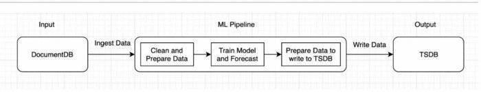
Our production pipeline needed to be capable of reading data from a DocumentDB, a TimeSeries DB, and In-stream data. Post preparing the data for modeling, training, and forecasting the outcome is finally written back to a TSDB. Negative forecasts are available via alerts for cluster admins on their customisable dashboards and on the various operational channels.

DocumentDB Sample Data

We use a DocumentDB to store data about all the components that we support and also resource usage values for each of the queues in YARN. Now, to analyze and write predictive algorithms about this data, the first step is to import this data for processing.

Below is a sample of sectional data looks like in raw form. This data is collected by our connectors for Acceldata supported components.

Each of the rows above describes the status of a queue at a particular point in time. Our main focus was to be to predict max capacity in the future.

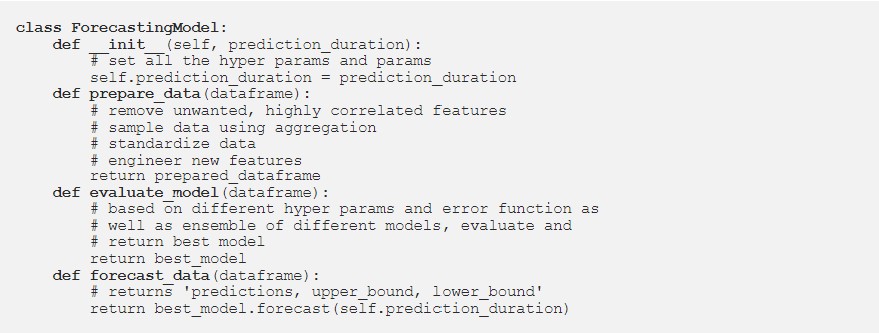
ML Pipeline

• Clean and Pre-process the data and get it ready to pass to a time-series model.
• Train the model and based on error criteria (discussed below), choose the best model
• Forecast predictions, upper bound as well as lower bounds
• Prepare data to write into TSDB

Cluster Admin Dashboard

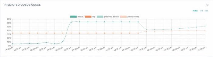
Finally, time to see the results! A Data Science project is incomplete without visualization. The predicted data that is pumped into the TSDB is rendered to the UI. The following images show 2 queues i.e. DEFAULT and LLAP which are sub-queues under the root queue. The first image merges the actual queue usage and predicted queue usage for the current day.

The second image is the predictions for the next day. The number of days to predict in the future is left as a configurable value available to Acceldata Administrators.

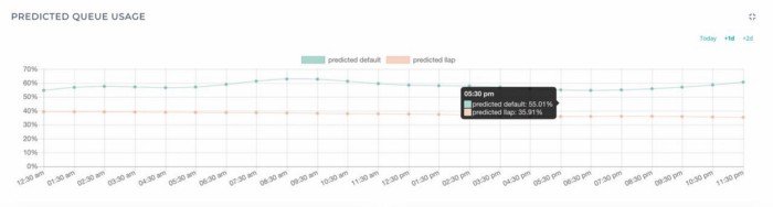
These models applied to customer-owned AWS environment predicted Yarn capacity usage in an error range of 3.5% of the actual values.

Impact

The accuracy of these predictions has given the customer a tremendous advantage in managing their AWS costs, as they can dynamically adjust their compute capacity.

ML Pipeline

Let’s see what all are the parts when stitched together help us get a Machine Learning model to production.

Data Engineering

There is enough material that discusses how Data Engineers extract data from different data sources, and therefore we will ignore that. We will simplify it to discuss how we performed data engineering instead.

• Data retrieval was a large effort and choices of SQL vs NoSQL vs warehouses, Batch vs Stream processing, made normalization very complex.
• For Acceldata, the data sources are a TSDB and a DocumentDB store. These data sources have Dataframe as the output format that we can fetch using the respective DB Clients for each. Above 95% of data points are numeric in nature.
• Using Dataframes and Numpy arrays makes it easy to run Machine Learning models due to the inherent support for these data types in most Machine Learning libraries

Now that we have our data extracted and ready for the Machine Learning model, let’s head into seeing what are the various parts in Machine Learning.

Machine Learning

1. Import Data

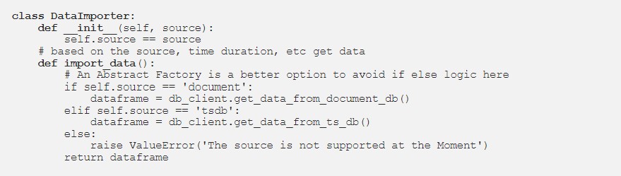
Once the data engineering (simply data ingestion) module is ready, data is imported, merged, and mutated into a DataFrame which is easier to work with Data Science workflows. The ML module now has the queue data in the DataFrames format.

Below is an example of how a Data Importer module looks.

2. Clean Data and Feature Engineering

As you might have heard more than a thousand times this is one of the most important aspects of Data Science

Some of the techniques we used are:

• Cleaning Unwanted Columns

- highly correlated data (noisy data)

- extra columns that may be passed by the data source

• Developing Useful Time Features

- day of the week/hour/month

- week of the month/year

- month/quarter of the year

- whether weekend or not

- proximity to weekend

• Normalising/Scaling Data

This is a very useful data preparation technique that improve results almost all the times when the values for different features do not fall in the same scale. It is just easy for the model to comprehend data that fit in the same scale.

• Sample Data

High-Frequency Metrics data (ms) is used for modeling. Therefore, it is important using aggregations like mean, median, min, max depending on the use-case. This enabled us to reduce noise from the signal.

Fit Data and Forecast

• Now that we have the data ready to be run the model on, we choose the “train and test data” and use multiple algorithms to observe which — Algorithms, hyper-params, and params give the best results.
• The best model is chosen and forecasts are then generated. Our models are an ensemble based on Facebook’s Prophet, LSTM, and VAR amongst others.

Below is a skeleton example of the Forecast Module along with the Data Preparation code looks.

Evaluation of the Models

Evaluation of Error Calculation is the measure that decides which model works better and should be chosen for forecasts on production data. Since we are dealing with absolute values, to avoid complicating this, we use MAPE as the error measure.

Currently, we see a +-5% error in the predictions and very rarely breach the threshold when there are unexpected workflows added, which will actually be considered when the model detects that there are changes that need to be fitted in the model. So, model refreshes and newer changes are accommodated.

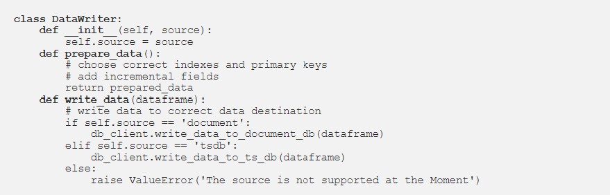
Prepare Data for Writing Results to DB

Data preparation is not only necessary to train the model but also to ensure that the Cluster Admins can make correct use of that data. Tasks are similar to:

• adding time as a field and in some cases even making it a primary key
• writing data keeping in mind the indexes for the tables/documents/measurements
• adding extra incremental fields in for charting & visualization

Below is an example of how the Data Writer looks.

TSDB

Now, most of the data that we collect at Acceldata is time-series based and it only makes sense to store it in a Time-Series database. Since the predictions are time-series based i.e. the forecasts are timestamps in the future displaying the queue usage, all the predictions are written to TSDB.

This is how the data in TSDB would look like:

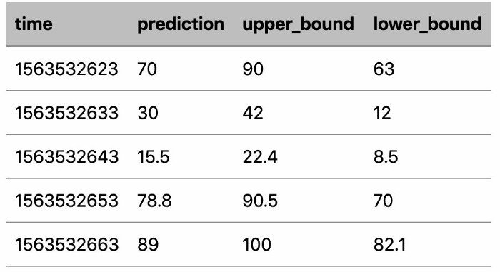
IMP: How to interpret the above results?

Let’s see what each of the fields above signify and how Acceldata adds value to the infrastructure.

• Prediction

The queue seems to be near full capacity in the 1st and 4th-time stamps. The administrator can make informed decisions as to whether she has to upscale the cluster or add more capacity. This is enforced by looking at the expected concurrency and number of jobs. However, the user has a good idea of whether he even needs to look at the above factors due to the predictions.

• Upper Bound, Lower Bound

We acknowledge the fact that accurate predictions about usage capacity are not an easy task. So, we also provide a upper_bound and lower_bound which states that these are the highest and lowest users can expect their queues to run at.

The upper bound cautions the user about a possible outage, the lower bound denotes under-utilised queues and that downscaling will lower TCO.

Bonus: This can be integrated with our Alerts framework thus letting the user know instead of monitoring the service. We even go further mentioning that we can take actions using the Auto-Actions framework so that the user need not spend time on trivial issues.

Data Model

We ask the cluster administrators to seed sampling, frequency, and prediction durations (remember we mentioned earlier accepting information from business users). So, it made sense to accept this kind of params to prepare our data or run our models based on them. This can be highly debated but suits our use case. Below is a sample of the request payload.

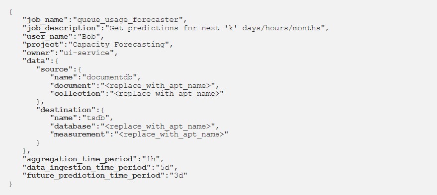
This can be persisted in a db to keep an account of the usage but again for brevity, we will skip discussing it.

Conclusion

Cost is an important factor that enterprises are wary of. Mission-critical data-intensive applications may suffer due to capacity issues when the provision is at the lower-bound of requirement, and costs swell when the provision is at the upper bound. Acceldata AIOps allows cluster administrators to lock-step with business needs without overspending. The above work dealt with right-sizing Hadoop clusters on AWS.

In the following post, we will discuss Acceldata auto-actions which enable Cloud Infrastructure Elasticity.

If you have elasticity challenges with your Data Applications, write to us product@acceldata.io.